Decipherment

Day 27: A New Decipherment

Today

• You will each be given a handout with a previously unknown text on it.
• Your task is to analyze the text and make as many observations as you can about it.
• You are encouraged to work with your neighbors.
• Write all observations on your handout.

Turn in your handout at the end of class for credit. You must work on the handout all class; otherwise you will receive partial credit.

Context

A previously unknown text was discovered in the basement of Funkhouser Hall, University of Kentucky.

• Location: Lexington, Kentucky
• Context: Buried beneath a stack of Linguistics handouts
• Language: unknown
• Type of Script: unknown
• Date of Composition: unknown

The Text

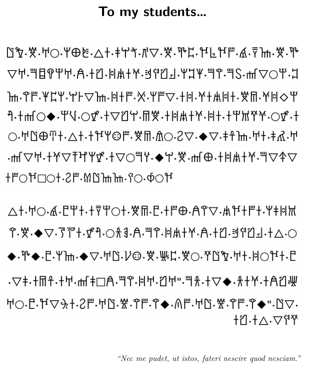
Your First Task

Your First Task (20 minutes)

• Linear Orientation
• Word Boundaries
• Symbol Inventory: approximately how many? Which symbols are most common?

Note: many Linear B symbols were used in the creation this activity, but their value has no bearing on the actual values in the text.

Further Investigation

Further Investigation (20 minutes)

• Find:
  • one very frequent symbol
  • one rare symbol
  • two repeated sequences (2–4 symbols)
  • at least two endings that appear on multiple words.
  • at least three words that occur more than once.

Further Investigation (20 minutes)

Find words that differ by only:

• one symbol at the end
  
• one symbol at the beginning

What might this variation mean?

Further Investigation (20 minutes)

Which type of system do you think it is? Choose one:

• Alphabet
• Syllabary
• Logographic
• Mixed

Justify your answer with evidence.

Crunching Some Numbers

Crunching Some Numbers (Remainder of Class)

• We’re now going to look at the text using some programming.
• I’ve done the work in “transliterating” the text using alphanumeric symbols, to make it a bit more computer friendly.

Google Colab

• Copy the transliterated text on slide 15, then visit the following website: https://colab.research.google.com/.
• Paste that code at the top of a new project, which you can call decipherment.ipynb

Character Mappings (for reference)

Each symbol in the original script has been replaced by a single character; word separators (·) and spaces between sentences are kept as-is.

| Code | Original | | Code | Original | | Code | Original |
|------|----------|-|------|----------|-|------|----------|
| A | □ | | B | △ | | C | ▽ |
| D | ◆ | | E | ◇ | | F | ○ |
| G | 𐀀 | | H | 𐀁 | | I | 𐀂 |
| J | 𐀃 | | K | 𐀄 | | L | 𐀅 |
| M | 𐀆 | | N | 𐀇 | | O | 𐀈 |
| P | 𐀉 | | Q | 𐀊 | | R | 𐀋 |
| S | 𐀍 | | T | 𐀎 | | U | 𐀏 |
| V | 𐀐 | | W | 𐀑 | | X | 𐀒 |
| Y | 𐀓 | | Z | 𐀔 | | a | 𐀕 |
| b | 𐀖 | | c | 𐀗 | | d | 𐀘 |
| e | 𐀙 | | f | 𐀚 | | g | 𐀛 |
| h | 𐀜 | | i | 𐀝 | | j | 𐀞 |
| k | 𐀟 | | l | 𐀠 | | m | 𐀢 |
| n | 𐀣 | | o | 𐀤 | | p | 𐀥 |
| q | 𐀦 | | r | 𐀨 | | s | 𐀩 |
| t | 𐀪 | | u | 𐀫 | | v | 𐀬 |
| w | 𐀭 | | x | 𐀮 | | y | 𐀯 |
| z | 𐀰 | | 0 | 𐀱 | | 1 | 𐀲 |
| 2 | 𐀴 | | 3 | 𐀵 | | 4 | 𐀶 |
| 5 | 𐀷 | | 6 | 𐀸 | | 7 | 𐀹 |
| 8 | 𐀺 | | 9 | 𐀼 | | + | 𐀽 |
| / | 𐀿 | | | | | | |

Transliterated Text

text = """JW·M·GF·sU+·Bu·jvc·8C·M·a1·drdx·7·eT·M·a1·fFCT·6x·nx·I1s·rJz+·wuyi·Ju·H·GfXQx·GCT·nx·I1s·vLCT·iux·R·sxC·ui·wuyiu·M5·wiEfu·WF·wgPfu·ui·wuyiu·M5·vJCu·WF·bf·DFTu·KF·GJUNu·Bu·udsox·M5·lF·6C·DC·j9T·Gu·jm·GC/Cx·wuyiu·UT·M·vD·qxFCu·Wsd3Cwu·GCT·uxFdAFu·6x·ZJTT·OF·4Fd

Bu·GF·7·0fu·uefFu·M5·0·uxU·HnC·yduxu·sjiPF·Bu·rJz+·Ju·H·wuyi·nx·H·ktF·KW·upS·CD·M·nD·aD·0·sT·DC·GJ·bo·M·h1·MF·gJW·Gu·iFdu·0hJHu·wut·DCu·tx·"GJ·Gi·nx·HAjT·Gu·95u·jC·GF·0·dCYu·6x·GJ·V·nx·nD·2x·GJ·V·nx·nD"·JC·gzC·Bu·Ju"""

print('Text loaded successfully!')
print(f'Total characters in text: {len(text)}')

You can copy the code by click on the box in the upper right-hand corner. Run this in your colab .ipynb document.

Splitting the text into words

In this script, words are separated by a middle dot (·). Let’s split the text into individual words.

# Split the text into words using the · separator
# We also strip out quotation marks so they don't interfere
clean_text = text.replace('"', '')
words = clean_text.split('·')

# Strip any extra spaces (from the paragraph break)
words = [w.strip() for w in words if w.strip()]

print(f'Total number of words (tokens): {len(words)}')
print()
print('First 10 words:')
for i, word in enumerate(words[:10]):
    print(f'  {i+1}. {word}')

Count Word Frequencies

Run this script to see how frequent words are. Remember, very frequent words are often grammatical words (like “the”, “and”, “of” in English).

from collections import Counter

word_counts = Counter(words)

print('=== WORD FREQUENCY (most common first) ===')
print(f'{"Word":<15} {"Count":<8} {"% of text"}')
print('-' * 35)

for word, count in word_counts.most_common(20):
    percentage = (count / len(words)) * 100
    print(f'{word:<15} {count:<8} {percentage:.1f}%')

print()
print(f'Total unique words (types): {len(word_counts)}')
print(f'Total word occurrences (tokens): {len(words)}')

Type-token Ratio (TTR)

The type-token ratio (TTR) tells us how varied the vocabulary is. (English prose is typically around 0.4–0.6.)

• A high TTR means almost every word is unique.
• A low TTR means many words are repeated.

num_types = len(word_counts)
num_tokens = len(words)
ttr = num_types / num_tokens

print(f'Unique words (types):   {num_types}')
print(f'Total words (tokens):   {num_tokens}')
print(f'Type-Token Ratio (TTR): {ttr:.3f}')
print()
if ttr > 0.7:
    print('High TTR: the vocabulary is quite varied for this text length.')
elif ttr > 0.4:
    print('Moderate TTR: a mix of repeated and unique words.')
else:
    print('Low TTR: many words are repeated frequently.')

Sign Frequencies

Now let’s count individual signs (characters). Frequent signs might be vowels, common consonants, syllables, words, or grammatical markers.

ignore = set('· "')
all_signs = [ch for ch in text if ch not in ignore]
sign_counts = Counter(all_signs)
total_signs = len(all_signs)

print('=== SIGN FREQUENCY (most common first) ===')
print(f'{"Sign":<8} {"Count":<8} {"% of signs"}')
print('-' * 30)

for sign, count in sign_counts.most_common():
    percentage = (count / total_signs) * 100
    print(f'{sign:<8} {count:<8} {percentage:.1f}%')

print()
print(f'Total signs: {total_signs}')
print(f'Unique signs: {len(sign_counts)}')

Positional Analysis

Some signs may prefer to appear at the beginning or end of words. This can reveal suffixes (like English -ing, -ed, -s) or prefixes.

initial_signs = [word[0] for word in words if len(word) > 0]
final_signs   = [word[-1] for word in words if len(word) > 0]

initial_counts = Counter(initial_signs)
final_counts   = Counter(final_signs)

print('=== MOST COMMON WORD-INITIAL SIGNS ===')
print(f'{"Sign":<8} {"Count":<8} {"% of words"}')
print('-' * 30)
for sign, count in initial_counts.most_common(10):
    pct = count / len(initial_signs) * 100
    print(f'{sign:<8} {count:<8} {pct:.1f}%')

print()
print('=== MOST COMMON WORD-FINAL SIGNS ===')
print(f'{"Sign":<8} {"Count":<8} {"% of words"}')
print('-' * 30)
for sign, count in final_counts.most_common(10):
    pct = count / len(final_signs) * 100
    print(f'{sign:<8} {count:<8} {pct:.1f}%')

Bigrams

A bigram is a pair of signs that appear next to each other within a word. Frequent bigrams can reveal common syllable patterns or repeated morphemes.

bigrams = []
for word in words:
    for i in range(len(word) - 1):
        bigrams.append(word[i] + word[i+1])

bigram_counts = Counter(bigrams)

print('=== MOST COMMON SIGN BIGRAMS ===')
print(f'{"Bigram":<10} {"Count":<8} {"% of bigrams"}')
print('-' * 32)
for bigram, count in bigram_counts.most_common(15):
    pct = count / len(bigrams) * 100
    print(f'{bigram:<10} {count:<8} {pct:.1f}%')

print()
print(f'Total bigrams: {len(bigrams)}')
print(f'Unique bigrams: {len(bigram_counts)}')

Word Length Distribution

How long are the words? This can give clues about whether the script is syllabic, alphabetic, or logographic.

word_lengths = [len(word) for word in words]
length_counts = Counter(word_lengths)
avg_length = sum(word_lengths) / len(word_lengths)

print('=== WORD LENGTH DISTRIBUTION ===')
print(f'{"Length":<10} {"Count":<8} Bar chart')
print('-' * 40)
for length in sorted(length_counts.keys()):
    count = length_counts[length]
    bar = '█' * count
    print(f'{length:<10} {count:<8} {bar}')

print()
print(f'Average word length: {avg_length:.2f} signs')
print(f'Shortest word: {min(word_lengths)} sign(s)')
print(f'Longest word:  {max(word_lengths)} sign(s)')

Plotting Sign Frequency

Let’s make a graph of sign frequencies.

Look at how many unique signs appear and how evenly their frequencies are distributed. Is the curve Zipfian?

import matplotlib.pyplot as plt

# Get sign frequencies in order
sign_freqs = [count for _, count in sign_counts.most_common()]

fig, axes = plt.subplots(1, 2, figsize=(14, 5))

# Left plot: frequency curve
axes[0].plot(range(1, len(sign_freqs) + 1), sign_freqs, color='coral', linewidth=2)
axes[0].set_xlabel('Sign rank (1 = most frequent)')
axes[0].set_ylabel('Frequency')
axes[0].set_title('Sign Frequency Distribution')

# Right plot: bar chart of all signs
signs  = [sign for sign, _ in sign_counts.most_common()]
counts = [count for _, count in sign_counts.most_common()]
axes[1].bar(range(len(signs)), counts, color='coral', alpha=0.8)
axes[1].set_xticks(range(len(signs)))
axes[1].set_xticklabels(signs, fontsize=8, rotation=45)
axes[1].set_xlabel('Sign')
axes[1].set_ylabel('Frequency')
axes[1].set_title('Frequency of Each Sign')

plt.tight_layout()
plt.show()

print(f'Total unique signs in this text: {len(sign_counts)}')
print()
print('What does the number of unique signs suggest about the script type?')
print('  < 30 signs  →  probably an alphabet')
print('  50-100 signs →  probably a syllabary')
print('  100+ signs  →  probably logographic')

So… what type of system is this?

1. Which type of system do you think it is?
2. Do you think this language primarily has prefixes or suffixes? And which signs/bigrams?
3. What are the three most common words? What do you think they might represent?